4 The subprime mortgage crisis unfolds in early 2007, part 2
Keywords: logistic regression, confusion matrix
4.1 The fall of FICO
The problem with the conventional wisdom of long standing is that it loses sight of history. The prominence of FICO in home loan credit underwriting described in the Pinto Testimony had its origins in a different time (the early 1990s) and a different lending environment. Freddie Mac was in a good position to ensure that all other things were equal. It made only what came to be called “prime” loans, generally for no more than 80% of the value of the property, under more stringent limitations on the debt-to-income ratio of the borrower and many other criteria that it kept within a narrow range, and offered only a few varieties of loans.
In the subprime market that emerged in the late 90s, all of those factors changed. Criteria that were narrow became broad, documentation was relaxed and a widespread assumption was that continually rising home values would preclude any problems. It’s not surprising that FICO lost its predictive power.
4.2 Overview of the down dependent variable
## Version:  1.36.23
## Date:     2017-03-03
## Author:   Philip Leifeld (University of Glasgow)
##
## Please cite the JSS article in your publications -- see citation("texreg").
##
## Attaching package: 'texreg'## The following object is masked from 'package:tidyr':
##
## extract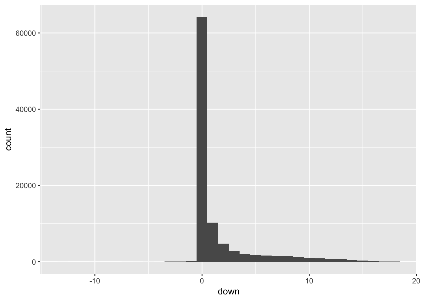
| deal | count |
|---|---|
| LBMLT 2006-1 | 18 |
| LBMLT 2006-10 | 18 |
| LBMLT 2006-11 | 25 |
| LBMLT 2006-2 | 40 |
| LBMLT 2006-3 | 21 |
| LBMLT 2006-4 | 34 |
| LBMLT 2006-5 | 18 |
| LBMLT 2006-6 | 26 |
| LBMLT 2006-7 | 21 |
| LBMLT 2006-8 | 23 |
| LBMLT 2006-9 | 27 |
| LBMLT 2006-WL1 | 17 |
| LBMLT 2006-WL2 | 32 |
| LBMLT 2006-WL3 | 33 |
MariaDB [dlf]> select down, count(down) from y7 group by down;
+------+-------------+
| down | count(down) |
+------+-------------+
|  -13 |           1 |
|  -10 |           1 |
|   -7 |           2 |
|   -6 |           3 |
|   -5 |           6 |
|   -4 |           4 |
|   -3 |          16 |
|   -2 |          67 |
|   -1 |         253 |
|    0 |       64229 |
|    1 |       10245 |
|    2 |        4724 |
|    3 |        2830 |
|    4 |        2074 |
|    5 |        1763 |
|    6 |        1627 |
|    7 |        1451 |
|    8 |        1470 |
|    9 |        1286 |
|   10 |        1019 |
|   11 |         852 |
|   12 |         728 |
|   13 |         600 |
|   14 |         448 |
|   15 |         306 |
|   16 |         160 |
|   17 |          88 |
|   18 |          18 |
+------+-------------+
Most of the loans are current – down = 0 – but a substantial number are in arrears by one or two payments or defaulted and in various stages of foreclosure.
The negative entries represent a few hundred loans that have made up to 13 months of advanced monthly payments (this was confirmed by checking a field in the database ptd, paid through date).
4.3 Logistic Regression
4.3.1 Restructuring the data
In this section we will be using logistic regression, for which we need a response variable that is binary, 1 or 0, performing or non-performing. This requires classifying the 28 values of down. I have chosen to classify two or fewer payments missed as performing (1), and three or more payments missed as non-performing (0). The binary performance variable will be named perf.
Some of the testing of FICO as a useful metric involved subsetting the data. There were many more variables than the ones used, some of them categorical and some categorical coded as numeric. Here is a summary of the remaining variables
| perf | count |
|---|---|
| 0 | 16,720 |
| 1 | 79,549 |
| grade | count |
|---|---|
| A | 6,886 |
| A- | 1,989 |
| A+ | 9,604 |
| AA | 2 |
| AP | 69,104 |
| AP+ | 2,573 |
| B | 2,039 |
| B- | 1 |
| B+ | 1,568 |
| C | 2,502 |
| D | 1 |
| purpose | count |
|---|---|
| Purchase | 62,077 |
| Refi - Cashout | 30,101 |
| Refi - No Cashout | 4,091 |
| dtype | count |
|---|---|
| Full | 52,580 |
| Limited | 3,789 |
| Stated | 39,900 |
| ltype | count |
|---|---|
| 2/28 LIBOR | 27,224 |
| 2/38 LIBOR | 22,602 |
| 2nd Fixed | 15,145 |
| 3/27 LIBOR | 3,564 |
| 3/37 LIBOR | 3,614 |
| 5/25 LIBOR | 4,303 |
| 5/35 LIBOR | 2,705 |
| 6 Month LIBOR | 51 |
| Fixed | 12,292 |
| I/O 2/28 LIBOR | 3,492 |
| I/O 3/27 LIBOR | 378 |
| I/O 3/37 LIBOR | 63 |
| I/O 5/25 LIBOR | 836 |
| otype | count |
|---|---|
| NOO | 11,197 |
| OO | 83,959 |
| sechome | 1,113 |
| ptype | count |
|---|---|
| 2-4 Units | 6,536 |
| Condo | 8,276 |
| PUD | 12,052 |
| SFR | 69,191 |
| Townhouse | 214 |
4.3.2 Creating training and testing subsets and their subsamples
The next step is to split the original dataset into a training set of approximately 2/3 of the data and a test set of the data and normalize the numeric data to prepare for testing.
This results in a training set with 64,212 and a test set with 46,697, each of which is a moderately largish dataset in its own right, so we will sample 12% of each to get reduced sets, a training sample of 7,705 and a test sample of 5,604.
4.3.3 Using the quantitative variables to predict loan performance with logistic regression
To start, we are going to return to the numeric variables, fico, dti, cltv, obal and orate. This time the dependent variable will not be continuous, as was down on the linear regression model, but binary, perf, with 1 for performing and 0 for non-performing. For this we use a generlized linear model on the sample of our training set.
| Estimate | Std. Error | z value | Pr(>|z|) | |
|---|---|---|---|---|
| (Intercept) | 1.753 | 0.03564 | 49.18 | 0 |
| fico | 0.1537 | 0.03649 | 4.213 | 2.524e-05 |
| dti | 0.05303 | 0.03312 | 1.601 | 0.1093 |
| cltv | -0.5646 | 0.05113 | -11.04 | 2.411e-28 |
| obal | -0.4729 | 0.03248 | -14.56 | 5.031e-48 |
| orate | -0.5118 | 0.03612 | -14.17 | 1.406e-45 |
All of the numeric variables have some degree of predictive power, except for dti.
Omitting dti yields
| Estimate | Std. Error | z value | Pr(>|z|) | |
|---|---|---|---|---|
| (Intercept) | 1.752 | 0.0356 | 49.23 | 0 |
| fico | 0.1475 | 0.03627 | 4.066 | 4.775e-05 |
| cltv | -0.55 | 0.05012 | -10.97 | 5.118e-28 |
| obal | -0.4682 | 0.03235 | -14.47 | 1.767e-47 |
| orate | -0.5151 | 0.03605 | -14.29 | 2.573e-46 |
4.3.4 Intepreting the results
4.3.4.1 How well does the training set self-classify?
Given the training model, we are going to turn it on itself through the predict function, which will give the probability for each loan of its perf being non-zero. This produces what is called a confusion matrix.
| 0 | 1 | |
|---|---|---|
| 0 | 23 | 22 |
| 1 | 1306 | 6354 |
The model classified 0.83 of the outcomes as having a greater than 50% probability of performing (*i.e., better than guessing). If we had set the bar at 75%, the results are similar: 0.82. Reaching for 80% accuracy, however, drops the results to 0.67.
4.3.4.2 Does the training model do as well on the test sample it hasn’t yet seen?
| 0 | 1 | |
|---|---|---|
| 0 | 12 | 16 |
| 1 | 942 | 4634 |
The training model does quite well on the test data. The model classified 0.83 of the outcomes as having a greater than 50% probability of performing (*i.e., better than guessing). If we had set the bar at 75%, the results are similar: 0.82. Reaching for 80% accuracy, however, drops the results to 0.68.
4.3.5 Next steps
We have a promising logistic model based on all of the quantitative variables but one, dti, that lacked predictive power. You could say, informally, that it has 75% accuracy. In the next installment, we will look at the effects of adding in the qualitative variables and move on to resampling and other cross validation methods.